Ocean freight volatility: planning MOQ and buffer stock

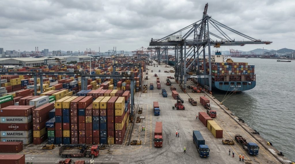
How container rates move: seasonality and shock events

Container rates out of Ningbo and Shanghai follow a recognizable seasonal pattern, and the pattern is routinely broken by events that no forecast captures. Demand typically builds from late July toward a peak in September and October as importers position stock for the western holiday season and the Lunar New Year factory shutdown. Rates soften in the first quarter and again in the early summer, although the exact timing shifts from year to year.

The shocks are what make planning difficult. Blank sailings, port congestion, equipment shortages, canal disruptions, fuel surcharges and geopolitical routing changes can move a rate by 40% to 300% within a few weeks. A single disruption on a major trade lane can pull capacity away from other lanes, so a buyer shipping to a secondary port may see rate volatility even when nothing happened on their own route.

The practical consequence is that a single annual freight assumption embedded in the landed cost is almost always wrong by the second half of the year. The more resilient approach is to plan rates as a distribution with a base case, a high case and a low case, and to make the procurement plan robust across that range rather than optimized for one point estimate.

The real cost of a late container versus the cost of carrying stock

A late container has a cost that is usually understated. The obvious components are expedited freight, air freight for the fastest-moving SKUs, overtime for the receiving team and, in the worst case, lost sales. The less obvious components are the downstream effects: a promotion that cannot be filled, a retail commitment that must be renegotiated, a distributor who starts qualifying a second supplier, and the management time spent firefighting.

Carrying stock has a cost too, and it is often overstated relative to the risk it mitigates. Inventory carrying cost for furniture typically runs 18% to 25% of product value per year, covering warehouse space, insurance, capital, damage and obsolescence. For a slow-moving item with a two-year life cycle, that cost can exceed the margin on the extra units. For a fast-moving item with stable demand, the calculation usually favors the buffer.

The correct comparison is the marginal cost of the extra week of cover against the marginal cost of a stockout. A common working figure is that a stockout costs 3 to 10 times the unit margin in lost future business, once customer defection is included. That asymmetry is why a moderate buffer on high-velocity SKUs is usually cheaper than a tight inventory posture, even when the carrying cost is calculated honestly.

Tiered procurement windows: base, seasonal and opportunistic layers

A tiered structure splits the annual volume into three layers. The base layer covers 50% to 60% of the forecast and is placed on a contract with a fixed rate and a fixed allocation, booked early enough to secure space on the desired sailings. The seasonal layer covers 20% to 30% and is booked once the demand signal for the season is clear, typically with a rate band rather than a fixed price. The opportunistic layer covers the remaining 10% to 20% and is placed when spot rates fall below the contract rate.

The base layer is insurance, not optimization. It will not be the cheapest rate of the year, and that is acceptable because it guarantees that the core assortment arrives. The seasonal layer is where most of the negotiation happens, and it benefits from being placed after the peak has been confirmed but before capacity tightens. The opportunistic layer requires the buyer to be able to receive goods on short notice, which means either ready warehouse space or a supplier who can hold finished goods for a defined period.

The layers should be defined by SKU velocity, not by an arbitrary split of the catalog. High-velocity, high-margin SKUs belong in the base layer; seasonal items belong in the seasonal layer; long-tail items that can tolerate a longer lead time belong in the opportunistic layer. Mixing the rules across the catalog is how a buyer ends up with a warehouse full of slow movers and a stockout on the best seller.

Calculating safety stock when lead time and demand are uncertain

The standard safety stock formula for independent demand is z multiplied by the square root of the sum of lead-time variance and demand variance, with the two terms scaled by average demand and average lead time respectively. The z value comes from the target service level: 1.28 for 90%, 1.65 for 95%, 2.33 for 99%. This formula is more realistic than the simpler average-demand-times-lead-time calculation because it accounts for the fact that both variables move.

For a furniture importer, lead-time variance is usually the larger term. A 35-day ocean leg can become 50 days with a blank sailing or a port backlog, and the variance grows further when the factory is running at capacity during peak season. If lead time is treated as a fixed 35 days, the resulting safety stock will cover normal demand variation and none of the schedule variation, which is where most stockouts originate.

The formula also assumes that demand is roughly normally distributed. For slow-moving SKUs with intermittent demand, a percentile-based or simulation-based method is more appropriate. Whichever method is used, the result should be reviewed against the actual fill rate. If the calculated safety stock produces a 92% fill rate against a 97% target, the inputs are wrong somewhere, and the variance estimates are the first place to look.

Warehousing options when a full container cannot be absorbed

Importers who cannot take a full container at once have three practical options. The first is a third-party warehouse near the port of discharge, which allows the factory to ship full containers while the importer draws stock in smaller lots. The second is a bonded warehouse, which defers duty until the goods are released, improving cash flow but adding administrative cost and storage fees. The third is to consolidate with other importers on a shared container, which reduces the unit cost of the ocean leg but adds coordination risk and a longer door-to-door schedule.

The choice depends on the ratio between the container cost and the warehouse cost. A 40-foot container from Ningbo to a US west coast port might carry a few thousand dollars of freight, while a month of third-party warehouse space for the same volume might cost a few hundred. When the destination warehouse is available at a reasonable rate, shipping full containers and drawing down inventory usually beats shipping partial loads at premium rates.

Contract structures that share the risk between buyer and factory

Freight risk can be shared in several ways. A fixed-rate contract puts all the risk on the carrier or forwarder and all the cost certainty on the buyer, which is simple but rarely available at favorable rates during peak season. A floating contract tied to a published index passes the risk to the buyer but keeps the price honest, and it is the most common structure for large annual volumes. A capped floating contract sets a ceiling and a floor, and is usually the best compromise for a mid-sized importer.

The negotiation should also cover who controls the booking, who chooses the sailing, who pays demurrage and detention, and what happens if the vessel is rolled. These clauses rarely matter in a normal month and always matter in a disrupted one. A contract that specifies the rate but not the allocation, the sailing window or the roll policy does not actually secure capacity.

Finally, the buyer should keep a current picture of the spot market even when shipping on contract. Spot rates are the best available signal of whether the contract rate is still competitive, and they provide leverage at renewal. A quarterly review of the rate against the index, the actual transit times and the fill rate turns freight from an annual negotiation into an ongoing procurement process, which is where most of the savings are actually found.